Mass conversion of SPSS files to CSV format in R
In this post, I provide a few options to convert large volume of SPSS data files to CSV files in R.
TLDR: In this rather long post, I provide a few options for mass conversion of SPSS data files to CSV, including steps to test out the functions on a simulated SPSS dataset. Assumes you already know the basics of working with R environment, including installing the packages where necessary.1
I’ve had to work with a large number of SPSS data files in my job lately, not an ideal scenario as I primarily use R for data processing/analysis. However, if you ever use secondary data, specially in social science disciplines, you are likely to come across survey data recorded in SPSS more often than not. SPSS has certainly been a mainstay of social science research, particularly those involving surveys, for as long as I can remember - I learned to use SPSS for the first time as an undergrad and that was over 2 decades ago (giving away my age here!). And it seems the software is still going strong. Digressions aside, I needed a way to easily convert all the SPSS files I had to open data formats like the CSV for better archiving and sharing.
As usual, I started by searching stackoverflow for mass conversion of SPSS to CSV in R, and found answers like this and a bit better version here. Both were useful in giving me ideas on what I wanted to do, but neither worked for me as they are. So, I decided to write my own function(s) to mass convert SPSS files to CSV in R. Below I outline three functions and highlight their pros and cons.
Function 1: Using convert() function from the rio package
RIO_SPSS2CSV <- function(filepath) {
  setwd(filepath) #this is the root dir where SPSS data files/folders are located; .csv files will be stored in the same dir
  library(rio)
  files <- list.files(path = filepath, pattern = '.sav', recursive = TRUE) #recursive option to check all folders inside the root dir
  for (f in files) {
    convert(f, paste0(strsplit(f, split = '.', fixed = TRUE)[[1]][1],'.csv'))
  }
}
This is the easiest and most straightforward of the three options I outline here. Basically the function above recursively looks for SPSS files within the specified filepath, and the uses the convert() function in rio package to convert them to CSV files in the same location. convert() basically wraps import() and export() functions thereby making the conversion simpler, however, not faster as we see below. It is also worth noting that this method writes values for the categorical variables rather than value labels (e.g., for variable sex in original SPSS data with 1=Female and 2=Male, CSV would have 1 or 2 under sex and not Female or Male), which means you’d need an extra variable definition file for categorical variable to fully understand converted CSV files.
Function 2: Using characterize() function together with import() and export() from the rio package
RIO_SPSS2CSV_VL <- function(filepath) {
  setwd(filepath)
  library(rio)
  files <- list.files(path = filepath, pattern = '.sav', recursive = TRUE)
  for (f in files) {
    export(characterize(import(f)), paste0(strsplit(f,split = '.', fixed = TRUE)[[1]][1],'.csv'))
  }
}
This is just a slight (but very useful) tweak in the previous option. It is still using rio package for the conversion, but instead of using convert() function, it now uses generic import() and export() functions with characterize() option to convert variables with defined value labels (i.e., categorical variables) to character or factor (e.g., for variable sex in original SPSS data with 1=Female and 2=Male, CSV would now have Female or Male under sex and not 1 or 2). This is particularly useful as you would not need a separate document defining value labels for categorical variables.
Function 3: Using foreign package with write.csv function
FOR_SPSS2CSV <- function(filepath) {
  setwd(filepath)
  files <- list.files(path = filepath, pattern = '.sav', recursive = TRUE)
  for (f in files) {
    write.csv(
      x = foreign::read.spss(file = f, to.data.frame = TRUE, use.value.labels = TRUE, use.missings = TRUE, reencode = FALSE),
      file = sprintf("%s.csv", tools::file_path_sans_ext(f)),
      row.names = FALSE, na = ""
      )
  }
}
This final option uses the foreign package, one of the default packages that comes with every R installation, so without the need to install any extra package for this task. Few good points about using foreign package — first, you can easily switch to copying values or value labels using the use.value.labels option (see function above); second, this gives you the option to define missing values in converted file using user defined missing values in SPSS by setting use.missings to TRUE; and finally, foreign provides warnings for unexpected values in original SPSS files, for example, when certain value in a categorical variable is undefined - allowing users to take actions against unexpected cases.
Testing the functions with simulated SPSS data
This section is really only possible because I found this excellent post on simulating SPSS data by Martin Chan. Example below is more or less literal copy from his post linked above - I’ve only tweaked the variable and data type to make them more relatable to the type of data with which I normally work.
Start by loading necessary packages - tidyverse, surveytoolbox and haven, and creating a directory to save simulated SPSS data file.
library(tidyverse)
library(surveytoolbox) #if you don't have this, you'll need to install it from the source with devtools::install_github("martinctc/surveytoolbox")
library(haven)
#create a directory to save simulated SPSS data. this will also be the base directory/filepath to test conversion functions above
dir.create("sav")
I want to simulate a more-or-less typical rural household survey data where majority of the household heads are male. So, I’m going to create a dataset with 200 observations with high male respondents in the sample - the dataset will have the variables sex (sex of HH head), education (highest education attainment of the HH head), and place_attach (place attachment). In addition, I’ll make education variable dependent on sex (with higher educational attainment skewed towards male HH heads); and place attachment variable dependent on highest educational attainment (those with higher education more likely to have lower place attachment).
Lets begin by creating id and sex variables.
set.seed(97) #this is to ensure reproducibility of this example but not necessary if simply testing SPSS to CSV conversion functions with your own data.

#id variable
v_id <- seq(1, 200) %>% set_varl("Household Identifier")

#sex variable
v_sex <- sample(x = 1:2,
                size = 200, replace = TRUE,
                prob = c(.25 , .75)) %>%  #skewed probability to reflect more male HH heads
  set_vall(value_labels = c("Female" = 1,
                            "Male" = 2)) %>%
  set_varl("HH Head's Sex")
Then create education variable that depends on sex variable above.
#Highest education attainment variable - sex-dependent sampling
v_edu <-
  v_sex %>%
  map_dbl(function(x){
    if(x == 1){
      sample(0:6,
             size = 1,
             prob = c(25, 15, 20, 20, 15, 5, 5)) #Sum to 100
    } else {
      sample(0:6,
             size = 1,
             prob = c(10, 10, 20, 15, 25, 10, 10)) #Sum to 100
    }
  }) %>%
  set_vall(value_labels = c("Illiterate" = 0,
                            "Literate - no formal education" = 1,
                            "Primary school" = 2,
                            "Lower secondary school" = 3,
                            "Secondary school" = 4,
                            "College/Technical college" = 5,
                            "University degree" = 6)) %>%
  set_varl("Highest education level")
Finally create variable for place attachment which depends on education variable above.
#Place attachment variable - education-dependent sampling
v_place <-
  v_edu %>%
  map_dbl(function(x){
    if(x>=4){
      sample(1:5,
             size = 1,
             prob = c(25, 25, 20, 20, 10)) #Sum to 100
    } else {
      sample(1:5,
             size = 1,
             prob = c(5, 10, 20, 30, 35)) #Sum to 100
    }
  }) %>%
  set_vall(value_labels = c("Not attached at all" = 1,
                            "Not very attached" = 2,
                            "Neutral" = 3,
                            "Attached" = 4,
                            "Very attached" = 5)) %>%
  set_varl("Place attachment")
You can now combine individual vectors and save the dataset2.
combined_df <-
  tibble(id = v_id,
         sex = v_sex,
         education = v_edu,
         place_attach = v_place)
Save the combined data to the new directory created at the beginning. And also create a couple of more SPSS files by subsetting the main simulated data so we have more than one file to check the conversion functions.
#save simulated data in SPSS format
combined_df %>% haven::write_sav("sav/Simulated_Dataset.sav")
#create more SPSS files from the same dataframe to test file conversion functions
combined_df %>% filter(sex==1) %>% write_sav("sav/female_only.sav")
combined_df %>% filter(sex==2) %>% write_sav("sav/male_only.sav")
Assuming the functions above are already loaded in your R environment, you simply load each function with the sav directory that you created at the beginning of simulated data creation in place of filepath as follows:
#using Function 1
RIO_SPSS2CSV("Drive://path/to/sav") #make sure you provide full file path as in the example, NOT relative path

#using Function 2
RIO_SPSS2CSV_VL("Drive://path/to/sav") #make sure you provide full file path as in the example, NOT relative path

#using Function 3
FOR_SPSS2CSV("Drive://path/to/sav") #make sure you provide full file path as in the example, NOT relative path
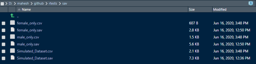
On every run of the above function, you’ll see SPSS files within your sav folder converted to CSV file with corresponding name, as shown in screenshot of my sav directory below:
Processing time and choice of option
I used tictoc package to get processing times for each of the functions. For the simulated data above, my processing times were 0.12s, 0.08s and 0.05s for Functions 1, 2 and 3 respectively. These functions were tested using R Version 4.0.1 in RStudio environment. I used Intel i7-6700 (3.4Ghz) with 32GB RAM and a SSD drive running Windows 10 for these tests. I also tested the functions on actual SPSS dataset. I had data from a very large household survey spread over multiple folders and files, each file with 160 to over 1000 observations (rows) and with five to over 50 variables (columns) in each file. Altogether 202 SPSS files were processed in 4 folders with directory structure as follows:
basedir
+--subfolder1
    +--subsubfolder1.1 (49 SPSS files, 3.47MB)
    +--subsubfolder1.2 (50 SPSS files, 4.36MB)
+--subfolder2
    +--subsubfolder2.1 (51 SPSS files, 5.72MB)
    +--subsubfolder2.2 (52 SPSS files, 5.46MB)
In terms of processing time (averaged over three runs for each function), Function 1 took the longest, followed by Function 3 — Function 2 being the fastest (see table below for summary).
| Function | Description | Processing time (seconds) |
|---|---|---|
| Function 1 | Function using convert() function from rio package. |
71.48 |
| Function 2 | Function using export() function in rio package with characterize() option to write value labels for categorical variables. |
52.10 |
| Function 3 | Function using foreign package to read SPSS files and write.csv() function to write CSV files. |
56.86 |
So, just looking at the processing time, obvious choice is to use Function 2. However, if you do like the options that foreign package provides to generate different outputs to account for different types of variables in SPSS, then you might still consider using Function 3 above, as the latter could be important especially for data from the social surveys.
To sum up, I think if you simply want to read SPSS files to work with them in R environment, using package like haven or rio which wraps haven among other packages within its functions provides you with better options to read and use metadata-rich formats like the SPSS. On the other hand, if you simply want to mass convert SPSS files to CSV files, you can pick Function 2 or Function 3, depending on the kind of data you have in SPSS and the options you require in the conversion.
-
Post updated on 16 June 2020 to include the section on simulated SPSS data. ↩
-
In order to keep this post at a manageable length, I’ve left out some of the checks and verification you can do on the simulated data in this post, which you can see in Martin’s post here. ↩