Cartographic desktop backgrounds

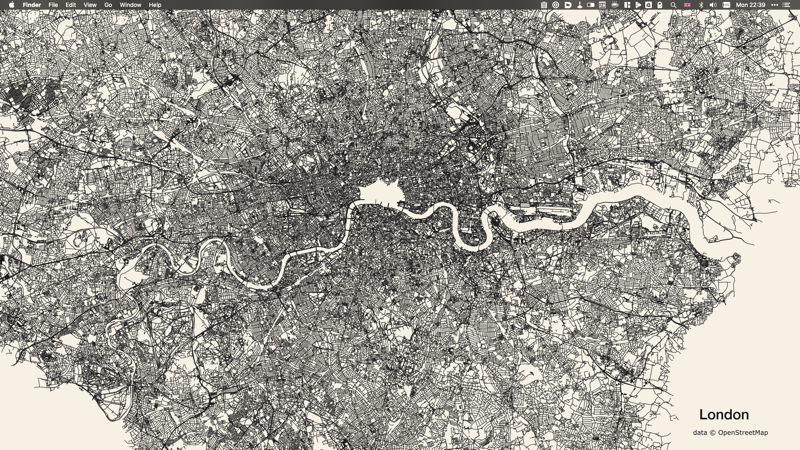
Inspired by this tweet and this tool that the tweet referred to, I tried to make my own cartographic desktop background for one of my monitors — for the second monitor I’m simply using the one I got for London using the above tool, which on my desktop looks like this:

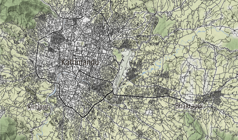
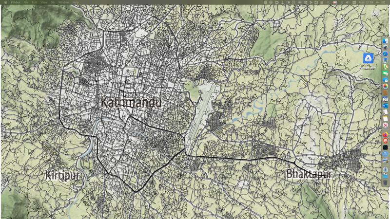
Below, I outline the steps in creating similar desktop background as above highlighting all the roads within a particular area but with a base map (e.g. terrain) instead of a plain background. I did one for Kathmandu and surrounding areas in Nepal in R using osmdata, sf and ggmap packages and looks like this:

First step, load the required libraries in R.

# load packages
library(osmdata)
library(tidyverse)
library(sf)
library(ggmap)

Next, get the base map outline and necessary map data from OSM. With the osmdata package, you are using ‘overpass API’ to extract OSM data. To get the map outline, you’ll have to define ‘bounding box’ - basically four coordinates/corners of your outline. If you just want to automatically create a ‘bounding box’ for a certain location, you can use getbb() function - for example, getbb("Kathmandu, Nepal"). However, I wanted to manually create a bounding box, for which I simply went to OSM webpage and used ‘Export’ feature to manually select the area I need to create bounding box coordinates that I used below. Once you have your bounding box, you then use opq() function to build the query. Finally, you use add_osm_feature() function in the query to add the feature you require in your map (in this case “highway”, which includes all the roads). Once you have the final query defined, you can use osmdata_sf() function to send the query defined earlier to the overpass server to return the data as a ‘simple feature (sf)’ format, which you’ll later plot. For the base map, you can use get_map() function from ggmap to pull the base map you want from among the options available.

# set bounding box
bb <- c(85.25, 27.64, 85.46, 27.75) #these coordinates bound Kathmandu and surrounding areas

# build query
q <- opq(bbox = bb) %>% 
  add_osm_feature("highway")

# get data in sf format
roads <- osmdata_sf(q)

# get base map, I'm using 'toner-background'
basemap <- get_map(bb, maptype = "toner-background")

You now have all the necessary things to produce the map. If you are familiar with ggplot functions, then the following steps should look familiar. First step below plots the base map, then adds the roads from the sf data (note you’ll have to specify ‘osm_lines’ from the dataframe). Finally, theme_void() option removes all the axes etc, to get a clean cartographic plot.

ggmap(basemap) + 
    geom_sf(data = roads$osm_lines,
            inherit.aes = FALSE) + 
    theme_void()

Output from above looks like this, which is my main monitor background shown earlier!